R Coding Exercise
Loading and checking the data
I first loaded the needed packages - dslabs to access the gapminder data and tidyverse to process the data and create plots.
I then loaded the help page for gapminder and asked for the structure, summary, and class.
#Load the dslabs and other required packages
#dslabs is required to access the gapminder data
library(dslabs)
#tidyverse is used in data processing and tidying and in plotting
library(tidyverse)
# gtsummary is for making nice regression tables in HTML output
library(gtsummary)
# For regression diagnostic plots
library(ggfortify)

#Look at the help file for the gapminder data
help(gapminder)

#Get an overview of the data structure
str(gapminder)
## 'data.frame': 10545 obs. of 9 variables:
## $ country : Factor w/ 185 levels "Albania","Algeria",..: 1 2 3 4 5 6 7 8 9 10 ...
## $ year : int 1960 1960 1960 1960 1960 1960 1960 1960 1960 1960 ...
## $ infant_mortality: num 115.4 148.2 208 NA 59.9 ...
## $ life_expectancy : num 62.9 47.5 36 63 65.4 ...
## $ fertility : num 6.19 7.65 7.32 4.43 3.11 4.55 4.82 3.45 2.7 5.57 ...
## $ population : num 1636054 11124892 5270844 54681 20619075 ...
## $ gdp : num NA 1.38e+10 NA NA 1.08e+11 ...
## $ continent : Factor w/ 5 levels "Africa","Americas",..: 4 1 1 2 2 3 2 5 4 3 ...
## $ region : Factor w/ 22 levels "Australia and New Zealand",..: 19 11 10 2 15 21 2 1 22 21 ...#Get a summary of the data
summary(gapminder)## country year infant_mortality life_expectancy
## Albania : 57 Min. :1960 Min. : 1.50 Min. :13.20
## Algeria : 57 1st Qu.:1974 1st Qu.: 16.00 1st Qu.:57.50
## Angola : 57 Median :1988 Median : 41.50 Median :67.54
## Antigua and Barbuda: 57 Mean :1988 Mean : 55.31 Mean :64.81
## Argentina : 57 3rd Qu.:2002 3rd Qu.: 85.10 3rd Qu.:73.00
## Armenia : 57 Max. :2016 Max. :276.90 Max. :83.90
## (Other) :10203 NA's :1453
## fertility population gdp continent
## Min. :0.840 Min. :3.124e+04 Min. :4.040e+07 Africa :2907
## 1st Qu.:2.200 1st Qu.:1.333e+06 1st Qu.:1.846e+09 Americas:2052
## Median :3.750 Median :5.009e+06 Median :7.794e+09 Asia :2679
## Mean :4.084 Mean :2.701e+07 Mean :1.480e+11 Europe :2223
## 3rd Qu.:6.000 3rd Qu.:1.523e+07 3rd Qu.:5.540e+10 Oceania : 684
## Max. :9.220 Max. :1.376e+09 Max. :1.174e+13
## NA's :187 NA's :185 NA's :2972
## region
## Western Asia :1026
## Eastern Africa : 912
## Western Africa : 912
## Caribbean : 741
## South America : 684
## Southern Europe: 684
## (Other) :5586#Determine the type of object gapminder is
class(gapminder)## [1] "data.frame"Processing the data
My first step was creating the new africadata object by filtering the gapminder dataset. I used only the rows for which the continent was Africa. I then checked the structure and summary of the new object.
I then created two additional objects from africadata, one containing only infant mortality and life expectancy data, and the other containing only population and life expectancy data. I checked the structures and summaries of these as well.
# Create a new object, "africadata," that contains only the data from African countries, by extracting only the rows from gapminder in which the continent is "Africa"
africadata <-
  gapminder %>%
  filter(continent == 'Africa')

#Check the structure and summary of the data
str(africadata)
## 'data.frame': 2907 obs. of 9 variables:
## $ country : Factor w/ 185 levels "Albania","Algeria",..: 2 3 18 22 26 27 29 31 32 33 ...
## $ year : int 1960 1960 1960 1960 1960 1960 1960 1960 1960 1960 ...
## $ infant_mortality: num 148 208 187 116 161 ...
## $ life_expectancy : num 47.5 36 38.3 50.3 35.2 ...
## $ fertility : num 7.65 7.32 6.28 6.62 6.29 6.95 5.65 6.89 5.84 6.25 ...
## $ population : num 11124892 5270844 2431620 524029 4829291 ...
## $ gdp : num 1.38e+10 NA 6.22e+08 1.24e+08 5.97e+08 ...
## $ continent : Factor w/ 5 levels "Africa","Americas",..: 1 1 1 1 1 1 1 1 1 1 ...
## $ region : Factor w/ 22 levels "Australia and New Zealand",..: 11 10 20 17 20 5 10 20 10 10 ...summary(africadata)## country year infant_mortality life_expectancy
## Algeria : 57 Min. :1960 Min. : 11.40 Min. :13.20
## Angola : 57 1st Qu.:1974 1st Qu.: 62.20 1st Qu.:48.23
## Benin : 57 Median :1988 Median : 93.40 Median :53.98
## Botswana : 57 Mean :1988 Mean : 95.12 Mean :54.38
## Burkina Faso: 57 3rd Qu.:2002 3rd Qu.:124.70 3rd Qu.:60.10
## Burundi : 57 Max. :2016 Max. :237.40 Max. :77.60
## (Other) :2565 NA's :226
## fertility population gdp continent
## Min. :1.500 Min. : 41538 Min. :4.659e+07 Africa :2907
## 1st Qu.:5.160 1st Qu.: 1605232 1st Qu.:8.373e+08 Americas: 0
## Median :6.160 Median : 5570982 Median :2.448e+09 Asia : 0
## Mean :5.851 Mean : 12235961 Mean :9.346e+09 Europe : 0
## 3rd Qu.:6.860 3rd Qu.: 13888152 3rd Qu.:6.552e+09 Oceania : 0
## Max. :8.450 Max. :182201962 Max. :1.935e+11
## NA's :51 NA's :51 NA's :637
## region
## Eastern Africa :912
## Western Africa :912
## Middle Africa :456
## Northern Africa :342
## Southern Africa :285
## Australia and New Zealand: 0
## (Other) : 0#Create an object containing only infant_mortality and life_expectancy data within the africadata object
v1 <- select(africadata, infant_mortality, life_expectancy)
#Create an object containing only population and life_expectancy data within the africadata object
v2 <- select(africadata, population, life_expectancy)
#Check the structure and summary of the two new objects
str(v1)## 'data.frame': 2907 obs. of 2 variables:
## $ infant_mortality: num 148 208 187 116 161 ...
## $ life_expectancy : num 47.5 36 38.3 50.3 35.2 ...summary(v1)## infant_mortality life_expectancy
## Min. : 11.40 Min. :13.20
## 1st Qu.: 62.20 1st Qu.:48.23
## Median : 93.40 Median :53.98
## Mean : 95.12 Mean :54.38
## 3rd Qu.:124.70 3rd Qu.:60.10
## Max. :237.40 Max. :77.60
## NA's :226str(v2)## 'data.frame': 2907 obs. of 2 variables:
## $ population : num 11124892 5270844 2431620 524029 4829291 ...
## $ life_expectancy: num 47.5 36 38.3 50.3 35.2 ...summary(v2)## population life_expectancy
## Min. : 41538 Min. :13.20
## 1st Qu.: 1605232 1st Qu.:48.23
## Median : 5570982 Median :53.98
## Mean : 12235961 Mean :54.38
## 3rd Qu.: 13888152 3rd Qu.:60.10
## Max. :182201962 Max. :77.60
## NA's :51Plotting
I created plots for each of the two new objects I created from africadata. Both had Life Expectancy as the outcome, while the first had infant mortality as the predictor and the second had the log population size as the predictor.
#Plot life expectancy as a function of infant mortality
v1 %>%
  ggplot(aes(infant_mortality, life_expectancy)) +
  geom_point() +
  xlab('Infant Mortality') +
  ylab('Life Expectancy')
## Warning: Removed 226 rows containing missing values (geom_point).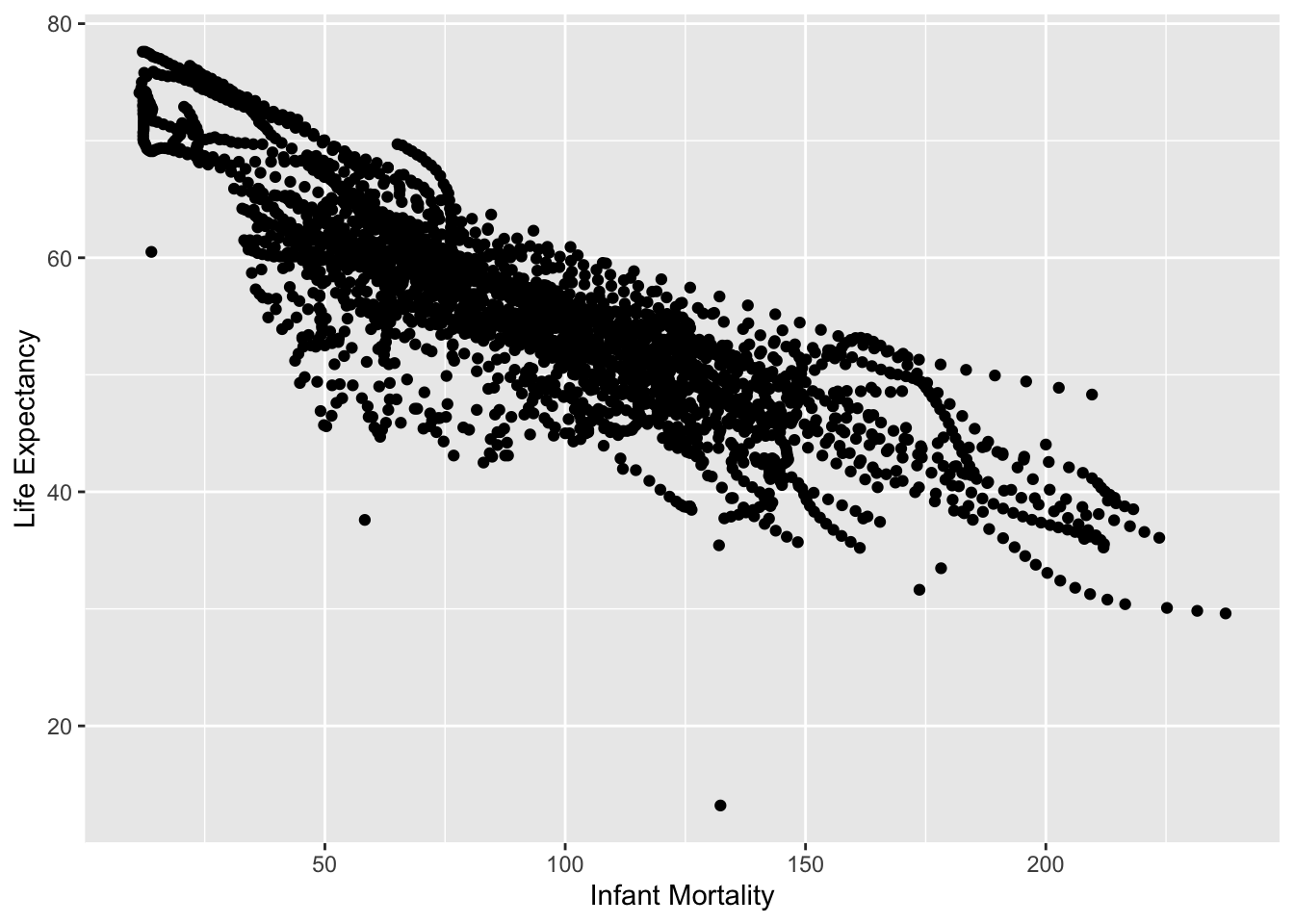
#Plot life expectancy as a function of the log population size
v2 %>%
  ggplot(aes(population, life_expectancy)) +
  scale_x_continuous(trans = 'log2') +
  geom_point() +
  xlab('Population (log scale)') +
  ylab('Life Expectancy')
## Warning: Removed 51 rows containing missing values (geom_point).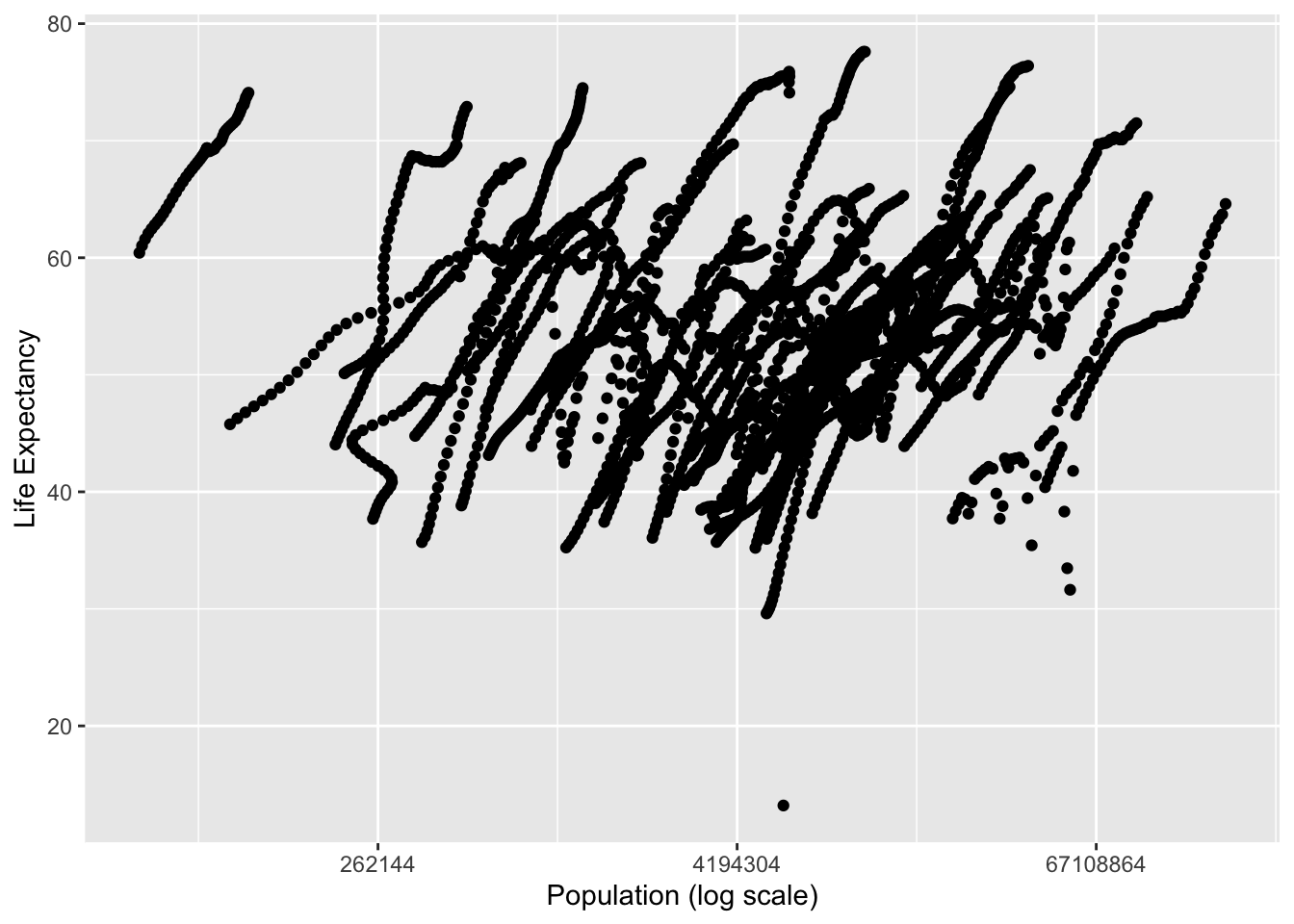
While these were scatter plots, they both had clusters of data points together that appeared almost linear. This was due to the data being collected over many different years. In order to tidy the data a little bit, the data was then restricted to one year.
More data processing
In order to determine which year to use, I examined what years containing missing data (so that I would avoid using a year with missing data).
The year 2000 was then used to go through the same process as above, in both processing and plotting data.
#Look at which years have missing data for infant mortality
africadatana <-
  africadata %>%
  select(year, infant_mortality) %>%
  filter(is.na(infant_mortality))
#1960-1981 and 2016 have missing data


#Creat new object with only the data from the year 2000 in the africadata object
africadata2000 <-
  filter(africadata, year == 2000)
#View the structure and summary of the new africadata2000 object
str(africadata2000)
## 'data.frame': 51 obs. of 9 variables:
## $ country : Factor w/ 185 levels "Albania","Algeria",..: 2 3 18 22 26 27 29 31 32 33 ...
## $ year : int 2000 2000 2000 2000 2000 2000 2000 2000 2000 2000 ...
## $ infant_mortality: num 33.9 128.3 89.3 52.4 96.2 ...
## $ life_expectancy : num 73.3 52.3 57.2 47.6 52.6 46.7 54.3 68.4 45.3 51.5 ...
## $ fertility : num 2.51 6.84 5.98 3.41 6.59 7.06 5.62 3.7 5.45 7.35 ...
## $ population : num 31183658 15058638 6949366 1736579 11607944 ...
## $ gdp : num 5.48e+10 9.13e+09 2.25e+09 5.63e+09 2.61e+09 ...
## $ continent : Factor w/ 5 levels "Africa","Americas",..: 1 1 1 1 1 1 1 1 1 1 ...
## $ region : Factor w/ 22 levels "Australia and New Zealand",..: 11 10 20 17 20 5 10 20 10 10 ...summary(africadata2000)## country year infant_mortality life_expectancy
## Algeria : 1 Min. :2000 Min. : 12.30 Min. :37.60
## Angola : 1 1st Qu.:2000 1st Qu.: 60.80 1st Qu.:51.75
## Benin : 1 Median :2000 Median : 80.30 Median :54.30
## Botswana : 1 Mean :2000 Mean : 78.93 Mean :56.36
## Burkina Faso: 1 3rd Qu.:2000 3rd Qu.:103.30 3rd Qu.:60.00
## Burundi : 1 Max. :2000 Max. :143.30 Max. :75.00
## (Other) :45
## fertility population gdp continent
## Min. :1.990 Min. : 81154 Min. :2.019e+08 Africa :51
## 1st Qu.:4.150 1st Qu.: 2304687 1st Qu.:1.274e+09 Americas: 0
## Median :5.550 Median : 8799165 Median :3.238e+09 Asia : 0
## Mean :5.156 Mean : 15659800 Mean :1.155e+10 Europe : 0
## 3rd Qu.:5.960 3rd Qu.: 17391242 3rd Qu.:8.654e+09 Oceania : 0
## Max. :7.730 Max. :122876723 Max. :1.329e+11
##
## region
## Eastern Africa :16
## Western Africa :16
## Middle Africa : 8
## Northern Africa : 6
## Southern Africa : 5
## Australia and New Zealand: 0
## (Other) : 0#Recreate v1 and v2 objects from the africa data in only the year 2000
#Create an object containing only infant_mortality and life_expectancy data within the africadata object
v1_2000 <- select(africadata2000, infant_mortality, life_expectancy)
#Create an object containing only population and life_expectancy data within the africadata object
v2_2000 <- select(africadata2000, population, life_expectancy)
#Check the structure and summary of the two new objects
str(v1_2000)## 'data.frame': 51 obs. of 2 variables:
## $ infant_mortality: num 33.9 128.3 89.3 52.4 96.2 ...
## $ life_expectancy : num 73.3 52.3 57.2 47.6 52.6 46.7 54.3 68.4 45.3 51.5 ...summary(v1_2000)## infant_mortality life_expectancy
## Min. : 12.30 Min. :37.60
## 1st Qu.: 60.80 1st Qu.:51.75
## Median : 80.30 Median :54.30
## Mean : 78.93 Mean :56.36
## 3rd Qu.:103.30 3rd Qu.:60.00
## Max. :143.30 Max. :75.00str(v2_2000)## 'data.frame': 51 obs. of 2 variables:
## $ population : num 31183658 15058638 6949366 1736579 11607944 ...
## $ life_expectancy: num 73.3 52.3 57.2 47.6 52.6 46.7 54.3 68.4 45.3 51.5 ...summary(v2_2000)## population life_expectancy
## Min. : 81154 Min. :37.60
## 1st Qu.: 2304687 1st Qu.:51.75
## Median : 8799165 Median :54.30
## Mean : 15659800 Mean :56.36
## 3rd Qu.: 17391242 3rd Qu.:60.00
## Max. :122876723 Max. :75.00More plotting
#Recreate plots with year 2000 data
###Plot life expectancy as a function of infant mortality
v1_2000 %>%
  ggplot(aes(infant_mortality, life_expectancy)) +
  geom_point()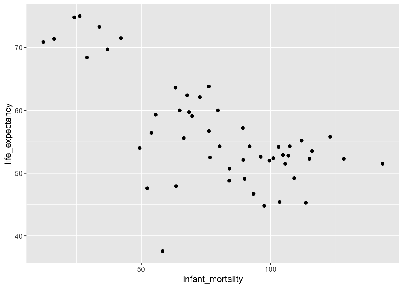
###Plot life expectancy as a function of the log population size
v2_2000 %>%
  ggplot(aes(population, life_expectancy)) +
  scale_x_continuous(trans = 'log2') +
  geom_point()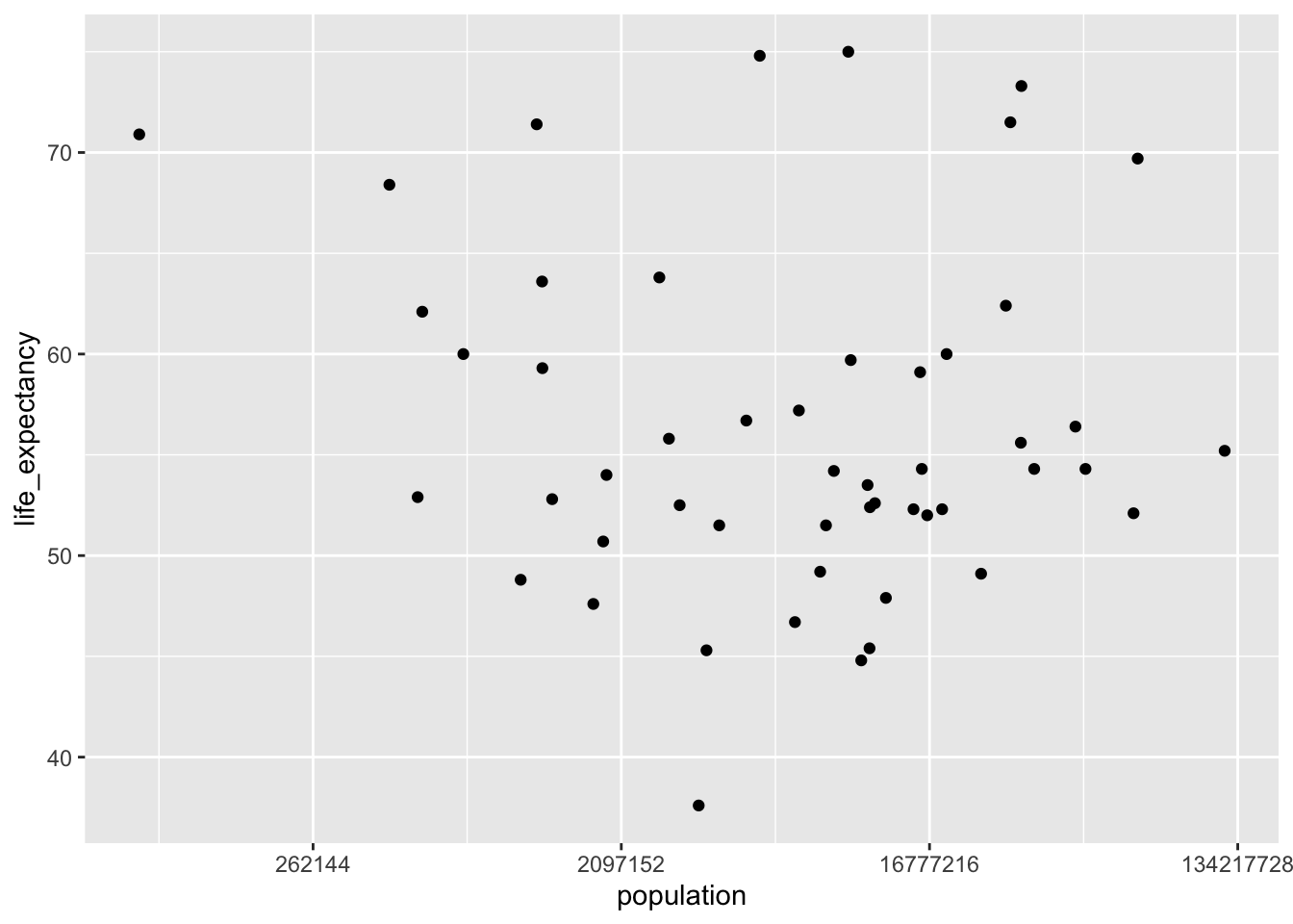
A simple fit
The data was now much more readable. There certainly appeared to be an association between infant mortality and life expectancy, but not much of one (if any) between population size and life expectancy. To check these relationships, two simple linear models were fit, one to each relationship.
#Fit linear models for the year 2000 data, with life expectancy as the outcome and infant mortality and population size as the predictors (separately), and save

## Linear model with infant mortality predictor and life expectancy outcome
fit1 <- lm(life_expectancy ~ infant_mortality, data = v1_2000)

## Linear model with (log) population size predictor and life expectancy outcome
fit2 <- lm(life_expectancy ~ population, data = v2_2000)

#View the summaries of the two linear models
summary(fit1)
##
## Call:
## lm(formula = life_expectancy ~ infant_mortality, data = v1_2000)
##
## Residuals:
## Min 1Q Median 3Q Max
## -22.6651 -3.7087 0.9914 4.0408 8.6817
##
## Coefficients:
## Estimate Std. Error t value Pr(>|t|)
## (Intercept) 71.29331 2.42611 29.386 < 2e-16 ***
## infant_mortality -0.18916 0.02869 -6.594 2.83e-08 ***
## ---
## Signif. codes: 0 '***' 0.001 '**' 0.01 '*' 0.05 '.' 0.1 ' ' 1
##
## Residual standard error: 6.221 on 49 degrees of freedom
## Multiple R-squared: 0.4701, Adjusted R-squared: 0.4593
## F-statistic: 43.48 on 1 and 49 DF, p-value: 2.826e-08summary(fit2)##
## Call:
## lm(formula = life_expectancy ~ population, data = v2_2000)
##
## Residuals:
## Min 1Q Median 3Q Max
## -18.429 -4.602 -2.568 3.800 18.802
##
## Coefficients:
## Estimate Std. Error t value Pr(>|t|)
## (Intercept) 5.593e+01 1.468e+00 38.097 <2e-16 ***
## population 2.756e-08 5.459e-08 0.505 0.616
## ---
## Signif. codes: 0 '***' 0.001 '**' 0.01 '*' 0.05 '.' 0.1 ' ' 1
##
## Residual standard error: 8.524 on 49 degrees of freedom
## Multiple R-squared: 0.005176, Adjusted R-squared: -0.01513
## F-statistic: 0.2549 on 1 and 49 DF, p-value: 0.6159Based on the outcomes of the two models, I could conclude that increased infant mortality has a negative impact on life expectancy. That is, as infant mortality increases, life expectancy decreases (p < 0.00001). However, there did not appear to be a significant relationship between life expectancy and population size (p = 0.616).
Predicting life expectancy (by Zane!)
What I want to do in this section is fit a basic model to predict life expectancy by year.
EDA
The first thing I want to do here is make a spaghetti plot of how each country’s life expectancy changes over the years.
africadata |>
  ggplot(aes(year, life_expectancy)) +
  geom_line(aes(color = country), alpha = 0.5, show.legend = FALSE) +
  geom_smooth(method = "gam", color = "black") +
  xlab('Infant Mortality') +
  ylab('Life Expectancy') +
  theme_bw()
## `geom_smooth()` using formula 'y ~ s(x, bs = "cs")'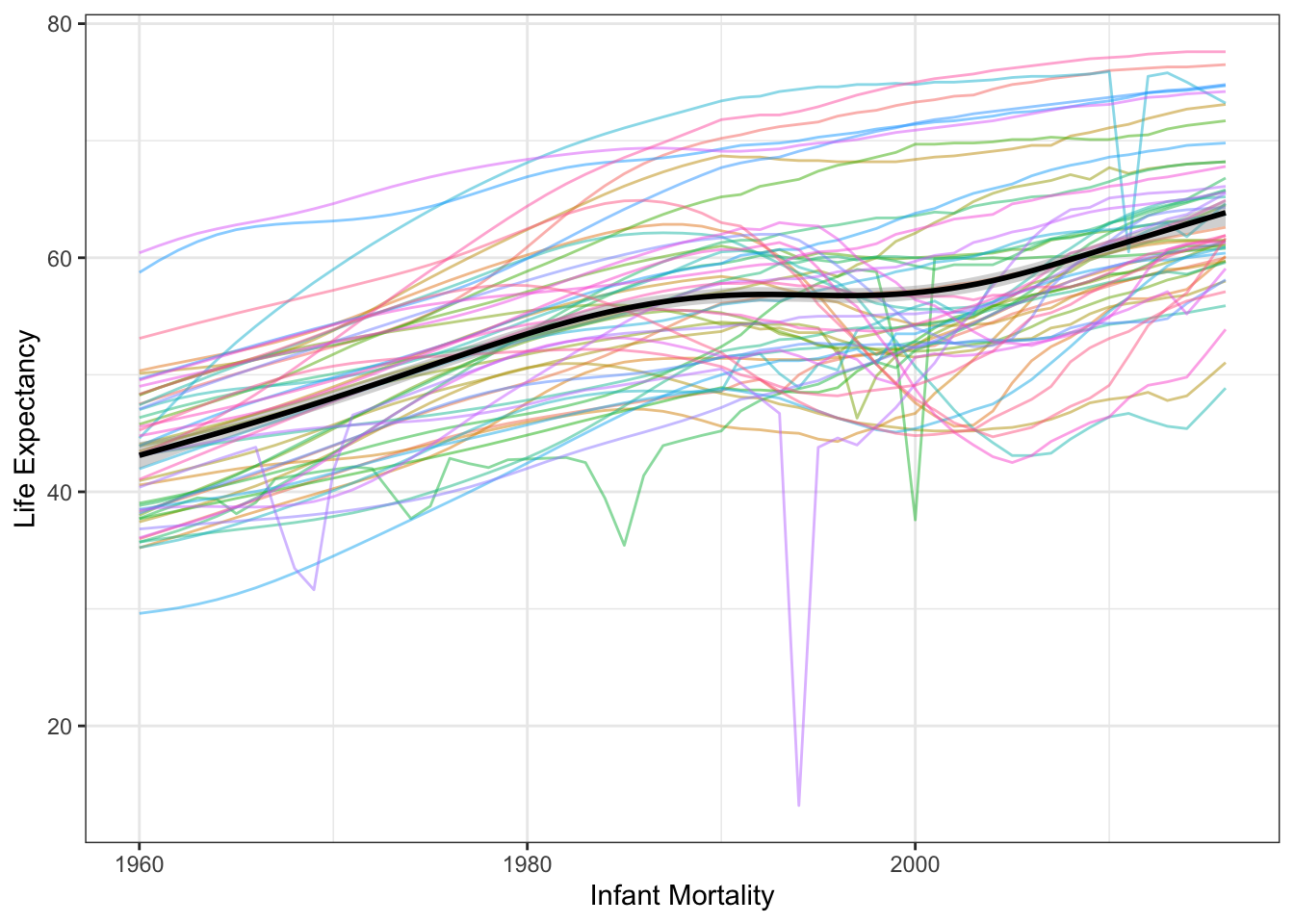
Hmm, it looks like this relationship is not monotonic for several countries, and while there is a trend upwards overall, it is not necessarily linear. There is also a significant amount of variation in the trend, which is pretty normal for time series. There doesn’t appear to be any seasonal/cyclic change, at least on the annual scale of measurement for which we have data.
Let’s color by region and see if we see any similar trends that could explain part of the country-level effect.
africadata |>
  ggplot(aes(year, life_expectancy)) +
  geom_line(aes(color = country), show.legend = FALSE, alpha = 0.5) +
  geom_smooth(method = "gam", color = "black") +
  xlab('Infant Mortality') +
  ylab('Life Expectancy') +
  theme_bw() +
  facet_wrap(vars(region))
## `geom_smooth()` using formula 'y ~ s(x, bs = "cs")'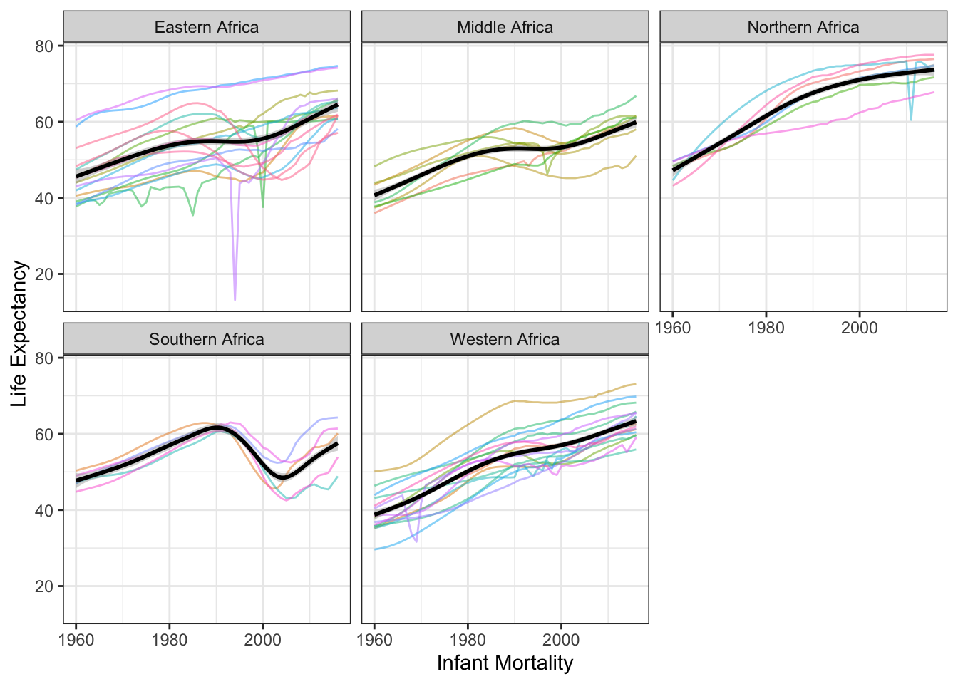
Let’s make a few more plots to see if we can observe any other relationships with life expectancy over time.
africadata |>
  mutate(`log10 population` = log10(population), `log10 gdp` = log10(gdp),
         .keep = "unused") |>
  pivot_longer(c(infant_mortality, fertility, `log10 population`,
                 `log10 gdp`)) |>
  ggplot(aes(year, value, color = life_expectancy, group = country)) +
  geom_line(alpha = 0.7) +
  scale_color_viridis_c(option = "plasma") +
  theme_bw() +
  coord_cartesian(expand = FALSE) +
  facet_wrap(vars(name), scales = "free_y")
## Warning: Removed 51 row(s) containing missing values (geom_path).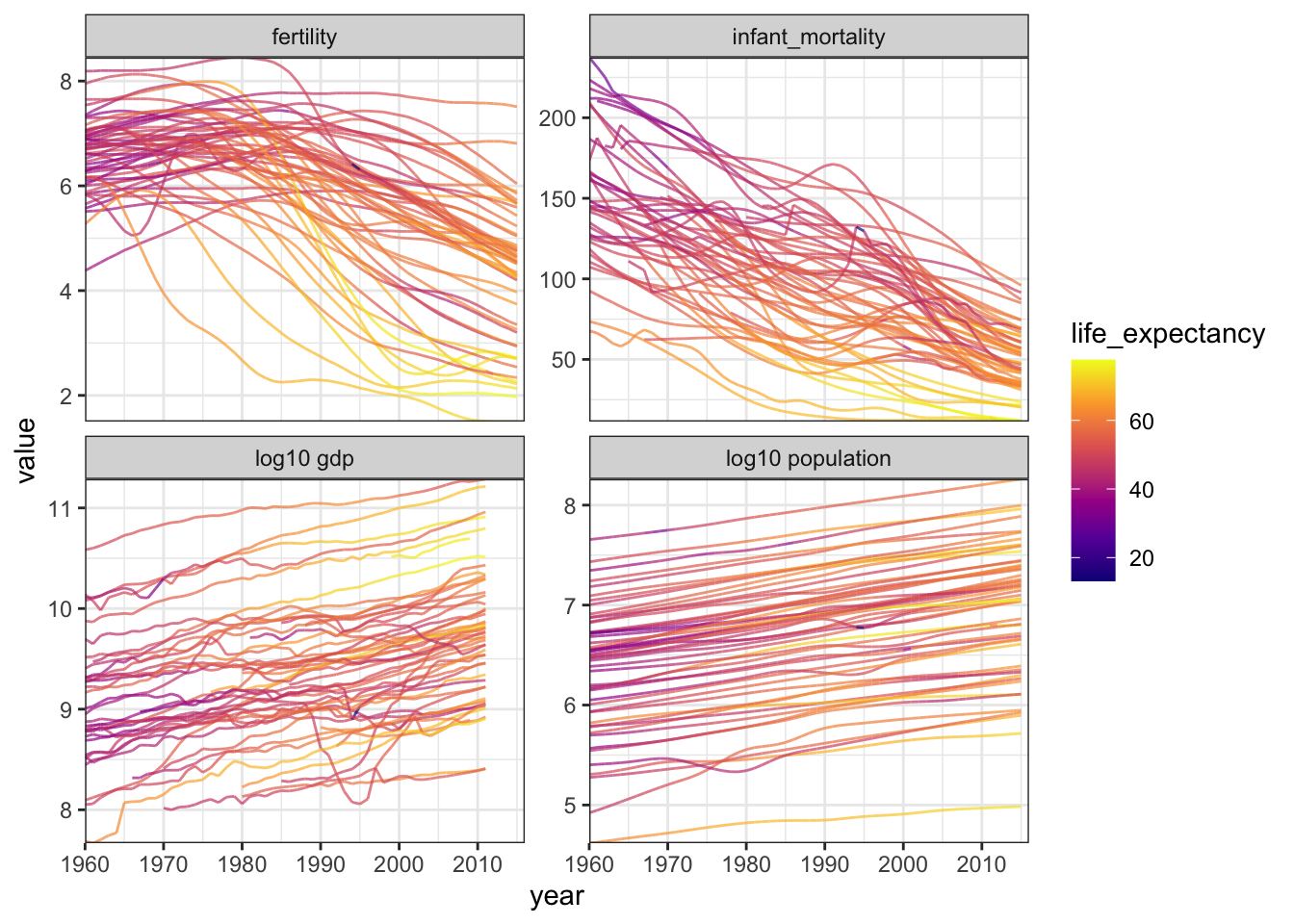
I won’t try and make the argument that this is the best possible visualization for these data, but I think it is good enough to give us an idea of trends. Clearly, fertility and infant mortality vary with life expectancy across time. We can see this from how the curves trend over time, and how the pattern of colors shifts over time. However, while gdp and population size appear to vary with time, I do not think that they necessarily vary with life expectancy in the same way.
Now since this is time series data, I think we are kind of obligated to plot the autocorrelation, so let’s make a plot of the partial autocorrelation (as this controls for previous lags, unlike the regular autocorrelation, and is thus easier to interpret).
africadata %>%
  select(country, year, life_expectancy) |>
  tidyr::nest(data = -country) |>
  dplyr::mutate(
    pacf_res = purrr::map(data, ~pacf(.x$life_expectancy, plot = F, lag.max = 10)),
    pacf_val = purrr::map(pacf_res, ~data.frame(lag = .x$lag, acf = .x$acf))
  ) |>
  unnest(pacf_val) |>
  ggplot(aes(x = lag, y = acf)) +
  geom_hline(yintercept = c(qnorm(0.025) / sqrt(17), qnorm(0.975) / sqrt(17)),
             lty = 2, color = "gray", size = 1.5) +
  geom_hline(yintercept = 0, size = 1.5) +
  geom_line(aes(group = country, color = country), show.legend = FALSE) +
  theme_bw(base_size = 20) +
  scale_x_continuous(labels = 1:10, breaks = 1:10, minor_breaks = NULL) +
  labs(x = "lag", y = "partial autocorrelation") +
  ggtitle("Partial autocorrelation of life expectancy by year for each African country")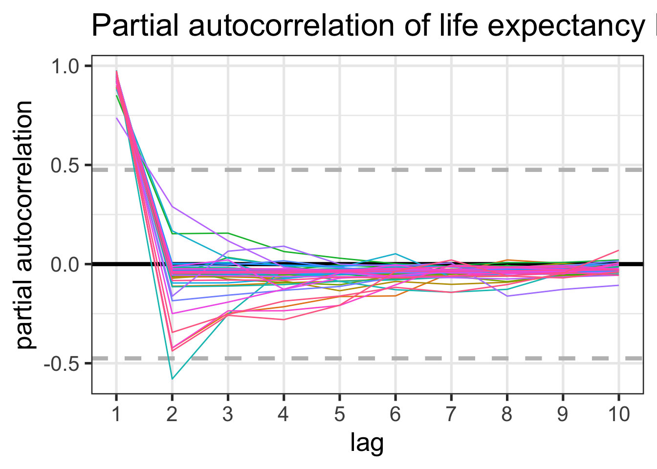
The dashed gray lines on this plot represent approximate normal 95% confidence bands. We see that all countries have a partial autocorrelation at the 1st lag which lies outside of the 95% confidence band, but at the 2nd lag, only one country has a value outside of the band. Since we are testing a larging amount of countries, I think we can safely say that this one second lag value is spurious. The interpretation of a significant first lag partial autocorrelation value (and no other significant partial autocorrelations) is that our time series can be modeled as an autoregressive process of order 1, AKA an AR(1) process.
Imputation
Most time series models have no way to deal with missing data. There are a lot of ways we could deal with this, and in this case we could likely find another data source to fill in the missing values with real information. But I am too lazy to do that. So first, let’s look at how much data is actually missing.
africadata |>
  select(!continent) |>
  summarize(across(everything(), ~mean(is.na(.x)))) |>
  pivot_longer(everything(), names_to = "field", values_to = "pct_m") |>
  ggplot(aes(x = pct_m, y = forcats::fct_reorder(field, pct_m))) +
  geom_col() +
  geom_label(aes(label = scales::percent(round(pct_m, 2))), size = 10) +
  theme_bw(base_size = 20) +
  labs(x = "percent of records missing", y = NULL) +
  scale_x_continuous(labels = scales::percent_format())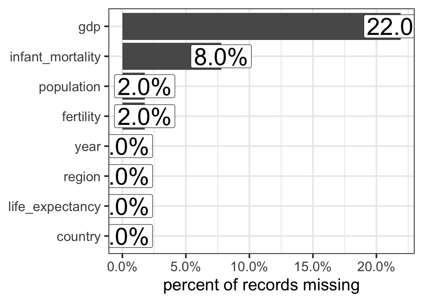
Well, the most missing values are in GDP, which did not appear to be a strong predictor anyways, so we can throw that one out. And then since infant mortality and fertility both have missingness less than 10%, for this simple example I think it will be fine to impute with the median, although in a real analysis something more complex might be better to reduce bias.
modeldata <- africadata |>
  dplyr::select(-continent, -gdp, -population) |>
  dplyr::mutate(
    across(c(infant_mortality, fertility),
           ~dplyr::if_else(is.na(.x), median(.x, na.rm = TRUE), .x)
           )
  )
Simple model fitting
Now that the imputation is done, let’s build a multivariable linear model. For this model we are going to ignore what we learned about the potentially autoregressive structure of the data :)
Now we have been looking at this by country previously, but I think that including 50+ regression parameters is maybe a bit excessive. So let’s group by region instead, which will give us a much more manageable number of regression coefficients. I don’t know which region of Africa we sould select as the reference group, so I will let R use the default (which in this case is Eastern Africa).
fit3 <- lm(life_expectancy ~ . - country, data = modeldata)
fit3 |>
  tbl_regression() |>
  add_glance_source_note(
    label = list(df  ~ "Degrees of Freedom", sigma ~ "\U03C3"),
    fmt_fun = df ~ style_number,
    include = c(r.squared, AIC, sigma, df)
)| Characteristic | Beta | 95% CI1 | p-value |
|---|---|---|---|
| year | 0.12 | 0.10, 0.13 | <0.001 |
| infant_mortality | -0.13 | -0.13, -0.12 | <0.001 |
| fertility | -0.32 | -0.49, -0.14 | <0.001 |
| region | |||
| Eastern Africa | — | — | |
| Middle Africa | -1.8 | -2.3, -1.3 | <0.001 |
| Northern Africa | 7.3 | 6.7, 7.9 | <0.001 |
| Southern Africa | -2.6 | -3.2, -1.9 | <0.001 |
| Western Africa | 0.69 | 0.25, 1.1 | 0.002 |
| R² = 0.745; AIC = 17,044; σ = 4.53; Degrees of Freedom = 7 | |||
|
1
CI = Confidence Interval
|
|||
We can see that all of the coefficients have low \(p\)-values, and the model has an \(R^2\) of 0.745 (that is, the linear model explains 74.5% of the variance in life expectancy), which is pretty good. Next we should at least glance at the diagnostics.
autoplot(fit3) + theme_bw()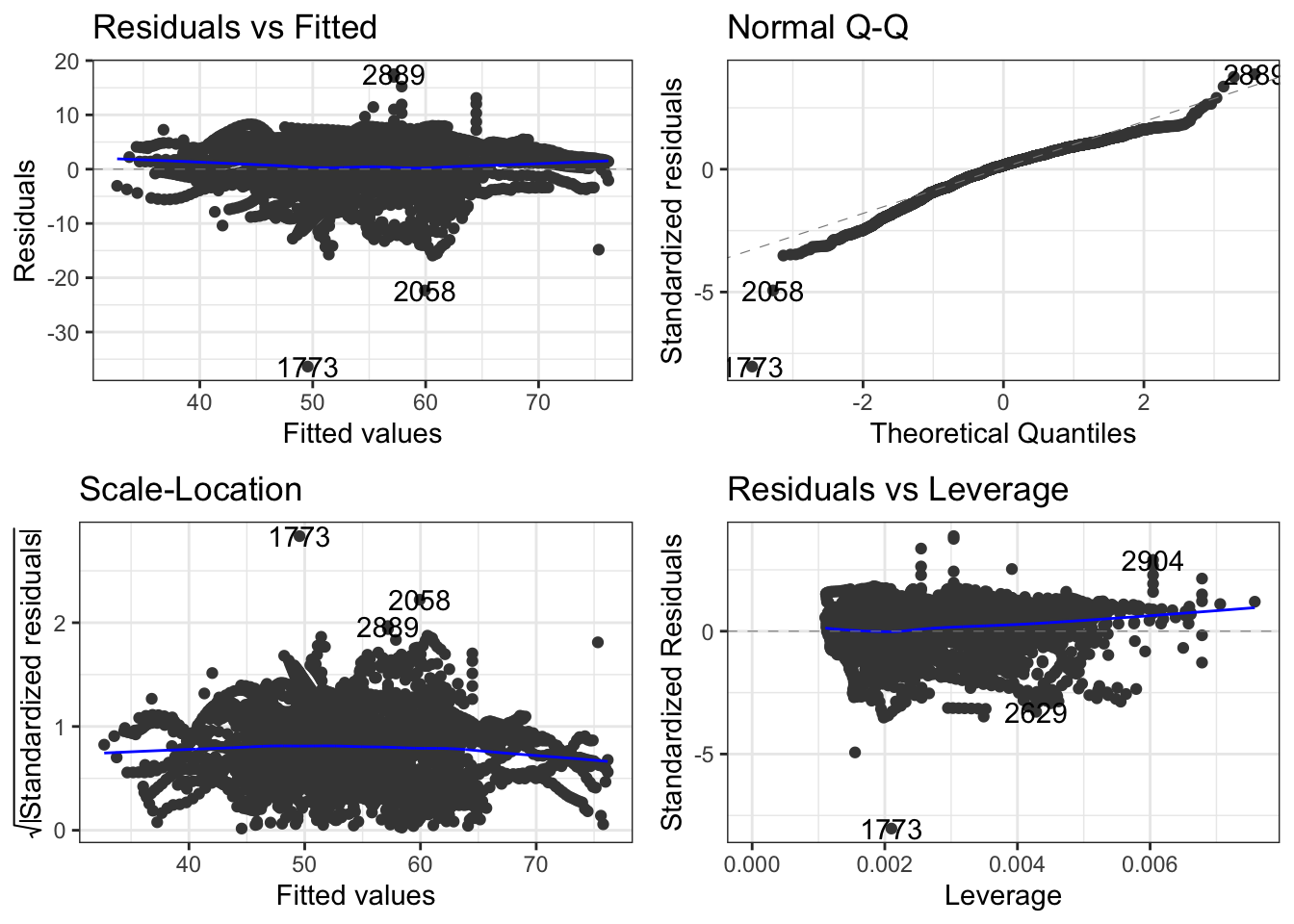
From the diagnostics, we can see minor deviations from normality and some evidence of non-constant variance in the residuals, but I think, similar to what we saw before, the plots indicate that the residuals are correlated, so we truly do need to correct for correlated residuals. This means that the standard errors (and thus reported confidence intervals) of the linear models we reported are not necessarily reliable under this model. Let’s plot the partial autocorrelations of the residuals for the model, this time using base R plotting for fun.
pacf(residuals(fit3))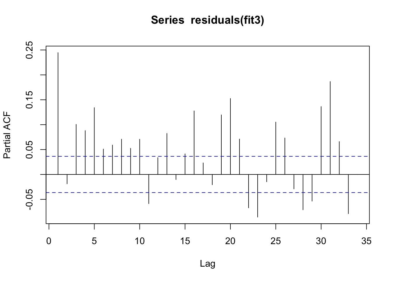
Yep, that is not ideal. There is definitely some residual autocorrelation of the residuals, though from this plot it is difficult to identify what the correlation structure is. So I think the next step would be adjusting for autocorrelation.
But I feel like this is long enough already, so I am just going to caution everyone about the weirdness that can show up with time series analysis and end this discussion here.