This is part of an analysis exercise in the Modern Applied Data Analysis course. The repository for the entire exercise can be found here.

Setup

I need to first load the packages we’ll be using and load in the data.

#load needed packages 
library(tidyverse) #for data processing

## ── Attaching packages ─────────────────────────────────────── tidyverse 1.3.1 ──

## ✓ ggplot2 3.3.5     ✓ purrr   0.3.4
## ✓ tibble  3.1.5     ✓ dplyr   1.0.7
## ✓ tidyr   1.1.4     ✓ stringr 1.4.0
## ✓ readr   2.0.2     ✓ forcats 0.5.1

## ── Conflicts ────────────────────────────────────────── tidyverse_conflicts() ──
## x dplyr::filter() masks stats::filter()
## x dplyr::lag()    masks stats::lag()

library(tidymodels) #for model fitting

## Registered S3 method overwritten by 'tune':
##   method                   from   
##   required_pkgs.model_spec parsnip

## ── Attaching packages ────────────────────────────────────── tidymodels 0.1.4 ──

## ✓ broom        0.7.9      ✓ rsample      0.1.0 
## ✓ dials        0.0.10     ✓ tune         0.1.6 
## ✓ infer        1.0.0      ✓ workflows    0.2.4 
## ✓ modeldata    0.1.1      ✓ workflowsets 0.1.0 
## ✓ parsnip      0.1.7      ✓ yardstick    0.0.8 
## ✓ recipes      0.1.17

## ── Conflicts ───────────────────────────────────────── tidymodels_conflicts() ──
## x scales::discard() masks purrr::discard()
## x dplyr::filter()   masks stats::filter()
## x recipes::fixed()  masks stringr::fixed()
## x dplyr::lag()      masks stats::lag()
## x yardstick::spec() masks readr::spec()
## x recipes::step()   masks stats::step()
## • Learn how to get started at https://www.tidymodels.org/start/

library(rsample) #for data splitting 
library(gtsummary) #for summary tables

## 
## Attaching package: 'gtsummary'

## The following object is masked from 'package:recipes':
## 
##     all_numeric

library(ranger) #for model fitting 
library(rpart) #for model fitting

## 
## Attaching package: 'rpart'

## The following object is masked from 'package:dials':
## 
##     prune

library(glmnet) #for model fitting

## Loading required package: Matrix

## 
## Attaching package: 'Matrix'

## The following objects are masked from 'package:tidyr':
## 
##     expand, pack, unpack

## Loaded glmnet 4.1-3

knitr::opts_chunk$set(echo = TRUE, message = FALSE, warning = FALSE)

#load data 
mydata <- readRDS(here::here('files', 'processeddata.rds'))

Feature/Variable Removal

I need to remove all Yes/No versions of variables that also exist as multiple level variables. Then, I need to code the three ordinal factors as ordered, in the proper order.

#remove yes/no version of multi-level variables - CoughYN, WeaknessYN, CoughYN2, MyalgiaYN
mydata.2 <- mydata %>% 
  select(!c(CoughYN, CoughYN2, WeaknessYN, MyalgiaYN))

#checking to see if ordinal factors are coded as ordered - Weakness, CoughIntensity, Myalgia
is.ordered(mydata.2$Weakness)

## [1] FALSE

is.ordered(mydata.2$CoughIntensity)

## [1] FALSE

is.ordered(mydata.2$Myalgia)

## [1] FALSE

#code ordinal/multi-level factors as ordered factors and check order is None/Mild/Moderate/Severe 
mydata.3 <- mydata.2 %>% 
  mutate(Weakness = ordered(Weakness, levels = c('None', 'Mild', 'Moderate', 'Severe'))) %>% 
  mutate(CoughIntensity = ordered(CoughIntensity, levels = c('None', 'Mild', 'Moderate', 'Severe'))) %>%
  mutate(Myalgia = ordered(Myalgia, levels = c('None', 'Mild', 'Moderate', 'Severe')))

#checking if new variables are coded as ordered 
is.ordered(mydata.3$Weakness)

## [1] TRUE

is.ordered(mydata.3$CoughIntensity)

## [1] TRUE

is.ordered(mydata.3$Myalgia)

## [1] TRUE

Low variance predictors

I now need to remove all binary predictors that have less than <50 entries in one of the categories. To do that, I first need to see what predictors fall into that category. Then I’ll remove them from the data set.

# create summary table to see what binary predictors have <50 in one category 
mydata.3 %>% 
  select(!c(Weakness, CoughIntensity, Myalgia, BodyTemp)) %>% #removing all non-binary predictors 
  gtsummary::tbl_summary() #create summary table

Characteristic	N = 730¹
Swollen Lymph Nodes	312 (43%)
Chest Congestion	407 (56%)
Chills/Sweats	600 (82%)
Nasal Congestion	563 (77%)
Sneeze	391 (54%)
Fatigue	666 (91%)
Subjective Fever	500 (68%)
Headache	615 (84%)
Runny Nose	519 (71%)
Abdominal Pain	91 (12%)
Chest Pain	233 (32%)
Diarrhea	99 (14%)
Eye Pain	113 (15%)
Sleeplessness	415 (57%)
Itchy Eyes	179 (25%)
Nausea	255 (35%)
Ear Pain	162 (22%)
Loss of Hearing	30 (4.1%)
Sore Throat	611 (84%)
Breathlessness	294 (40%)
Tooth Pain	165 (23%)
Blurred Vision	19 (2.6%)
Vomiting	78 (11%)
Wheezing	220 (30%)
¹ n (%)

# binary predictors with <50 in one category: Loss of Hearing, Blurred Vision
# need to remove those two variables 
mydata.4 <- mydata.3 %>% 
  select(!c(Hearing, Vision))

# Should have 730 observations and 26 variables - checking 
dim(mydata.4) #this looks right!

## [1] 730  26

# setting to final object name 
mydata.fin <- mydata.4

Data setup

In this step, I will set the seed to fix random numbers, split the data into train and test data, create and 5x5 cross-validation resample object, and create the recipe for the body temperature outcome as well as the linear regression model specification.

# set seed to fix random numbers 
set.seed(123)

# put 70% of data into training set 
data_split <- initial_split(mydata.fin, 
                            prop = 7/10, #split data set into 70% training, 30% testing
                            strata = BodyTemp) #use bodytemp as stratification 

# create data frames for training and testing sets 
train_data <- training(data_split)
test_data <- testing(data_split)

# create a resample object for the training data; 5x5, stratify on bodytemp 
cv5 <- vfold_cv(train_data, 
                v = 5, 
                repeats = 5, 
                strata = BodyTemp)

# create a recipe for the data and fitting; code categorical variables as dummy variables
temp_rec <- recipes::recipe(BodyTemp ~ ., 
                            data = train_data) %>% 
  step_dummy(all_predictors())

# linear model specification 
linear_reg_lm_spec <-
  linear_reg() %>%
  set_engine('lm')

Null model performance

The first model to fit is the null model. This will be fit to both the train and the test data.

#compute the performance of a null model with no predictor information - train data 
null_mod_train <- lm(BodyTemp ~ 1, data = train_data)
summary(null_mod_train)

## 
## Call:
## lm(formula = BodyTemp ~ 1, data = train_data)
## 
## Residuals:
##     Min      1Q  Median      3Q     Max 
## -1.6364 -0.7364 -0.4364  0.3636  4.1636 
## 
## Coefficients:
##             Estimate Std. Error t value Pr(>|t|)    
## (Intercept) 98.93642    0.05371    1842   <2e-16 ***
## ---
## Signif. codes:  0 '***' 0.001 '**' 0.01 '*' 0.05 '.' 0.1 ' ' 1
## 
## Residual standard error: 1.211 on 507 degrees of freedom

mean(train_data$BodyTemp) #checking the mean of body temp is the same as the bodytemp coefficient in the null model

## [1] 98.93642

#calculate RMSE 
null_mod_train %>% 
  augment(newdata = train_data) %>% 
  rmse(truth = BodyTemp, estimate = .fitted)

## # A tibble: 1 × 3
##   .metric .estimator .estimate
##   <chr>   <chr>          <dbl>
## 1 rmse    standard        1.21

#compute the performance of a null model with no predictor information - test data 
null_mod_test <- lm(BodyTemp ~ 1, data = test_data)
summary(null_mod_test)

## 
## Call:
## lm(formula = BodyTemp ~ 1, data = test_data)
## 
## Residuals:
##    Min     1Q Median     3Q    Max 
## -1.732 -0.732 -0.432  0.368  4.068 
## 
## Coefficients:
##             Estimate Std. Error t value Pr(>|t|)    
## (Intercept) 98.93198    0.07825    1264   <2e-16 ***
## ---
## Signif. codes:  0 '***' 0.001 '**' 0.01 '*' 0.05 '.' 0.1 ' ' 1
## 
## Residual standard error: 1.166 on 221 degrees of freedom

mean(test_data$BodyTemp) #checking the mean of body temp is the same as the bodytemp coefficient in the null model

## [1] 98.93198

#calculate RMSE 
null_rmse <- null_mod_test %>% 
  augment(newdata = test_data) %>% 
  rmse(truth = BodyTemp, estimate = .fitted) %>% 
  mutate(model = 'Null Model')

Model tuning and fitting

The model fitting process will be:

Define the model specification
Create a workflow
Create a tuning grid and tune the hyperparameters
Autoplot the results
Finalize the workflow
Fit the model to the training data
Estimate model performance with RMSE
Make diagnostic plots

Do these steps for each model (tree, LASSO, random forest)

Finally, look at RMSEs for all models (including null) together - choose best performing model, fit to test data, then repeat 7 and 8.

Tree

As a reminder, the tree model will be fit by following these steps:

Define the model specification
Create a workflow
Create a tuning grid and tune the hyperparameters
Autoplot the results
Finalize the workflow
Fit the model to the training data
Estimate model performance with RMSE
Make diagnostic plots

Let’s get started!

# 1) define model spec 
tree_tune_spec <- decision_tree(
  cost_complexity = tune(),
  tree_depth = tune()) %>% 
  set_engine('rpart') %>% 
  set_mode('regression')
tree_tune_spec

## Decision Tree Model Specification (regression)
## 
## Main Arguments:
##   cost_complexity = tune()
##   tree_depth = tune()
## 
## Computational engine: rpart

# 2) workflow 
tree_wflow <- workflow() %>% 
  add_model(tree_tune_spec) %>% 
  add_recipe(temp_rec)


# 3) create tuning grid 
tree_grid <- grid_regular(cost_complexity(),
                          tree_depth(),
                          levels = 5)

# tune hyperparameters 
tree_res <- tree_wflow %>% 
  tune_grid(resamples = cv5,
            grid = tree_grid,
            metrics = metric_set(rmse),
            control = control_grid(verbose = T))

# 4) autoplot the results 
tree_res %>% autoplot()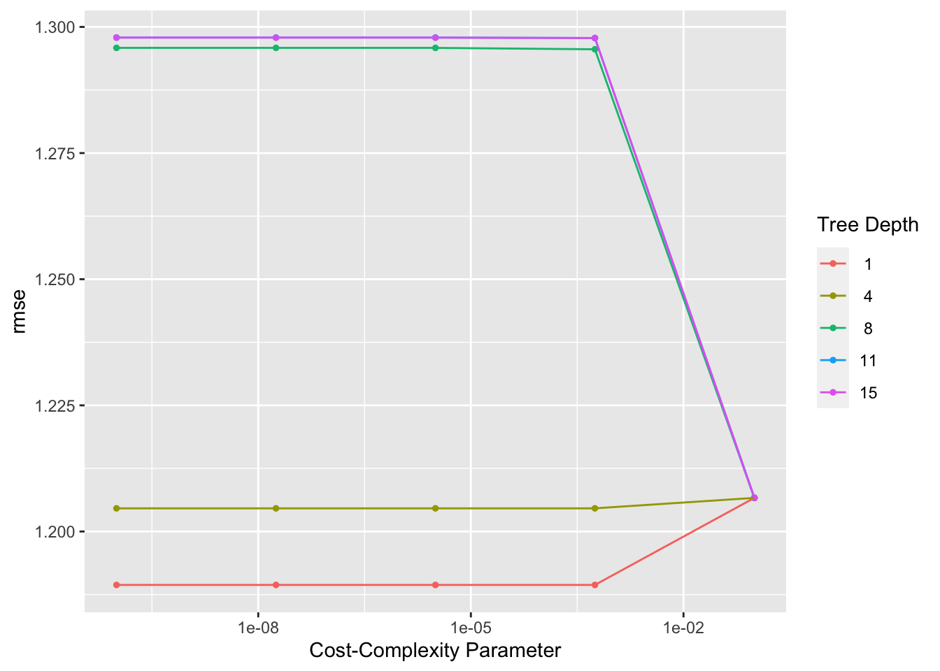

# 5) finalize the workflow 
## select best hyperparameter combination 
happy_tree <- tree_res %>% 
  select_best()
happy_tree

## # A tibble: 1 × 3
##   cost_complexity tree_depth .config              
##             <dbl>      <int> <chr>                
## 1    0.0000000001          1 Preprocessor1_Model01

## finalize workflow 
happy_tree_wflow <- tree_wflow %>% 
  finalize_workflow(happy_tree)

fit_train_happy_tree <- happy_tree_wflow %>% 
  fit(data = train_data)

# 6) fit the model to training data 
# Use a trained workflow to predict section using test data
predict(fit_train_happy_tree, new_data = train_data)

## # A tibble: 508 × 1
##    .pred
##    <dbl>
##  1  99.2
##  2  99.2
##  3  98.7
##  4  98.7
##  5  98.7
##  6  98.7
##  7  98.7
##  8  99.2
##  9  99.2
## 10  99.2
## # … with 498 more rows

# include predicted probabilities
aug_train_happy_tree <- augment(fit_train_happy_tree, new_data = train_data)

# 7) estimate model performance with rmse 
tree_rmse <- aug_train_happy_tree %>% 
  rmse(truth = BodyTemp, .pred) %>% 
  mutate(model = 'Regression Tree')
tree_rmse

## # A tibble: 1 × 4
##   .metric .estimator .estimate model          
##   <chr>   <chr>          <dbl> <chr>          
## 1 rmse    standard        1.18 Regression Tree

# 8) Make diagnostic plots 
## view decision tree 
extract_fit_engine(fit_train_happy_tree) |> rpart.plot::rpart.plot(digits = 4)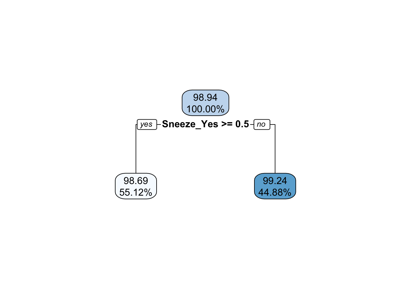

#plot actual vs fitted  
ggplot(data = aug_train_happy_tree, aes(x = .pred, y = BodyTemp)) +
  geom_point()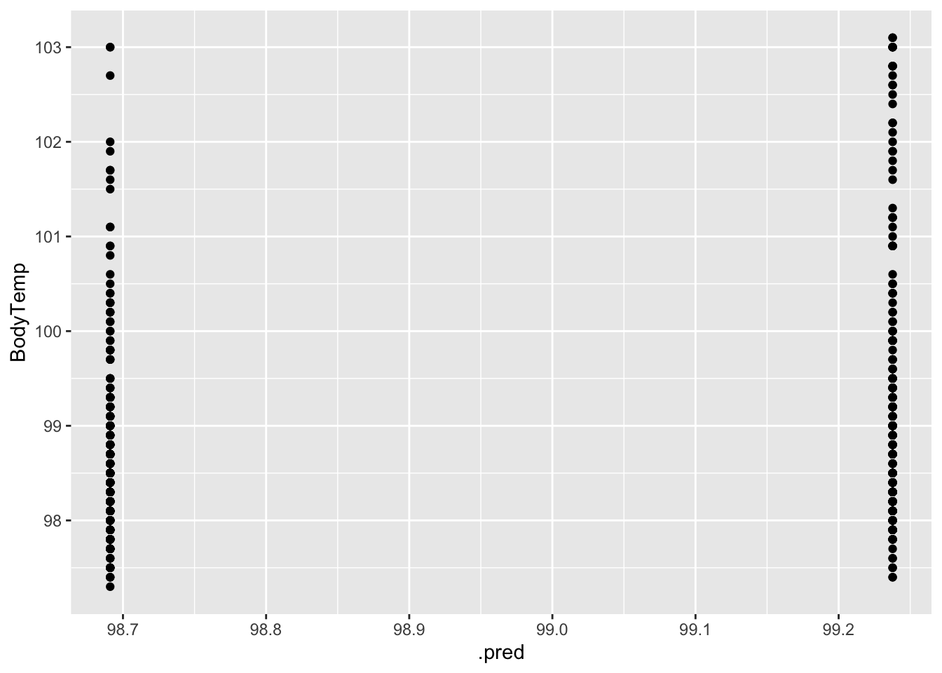

#plot residuals vs fitted 
aug_train_happy_tree %>% 
  mutate(resid = BodyTemp - .pred) %>% 
  ggplot(aes(x = .pred, y = resid)) +
  geom_point()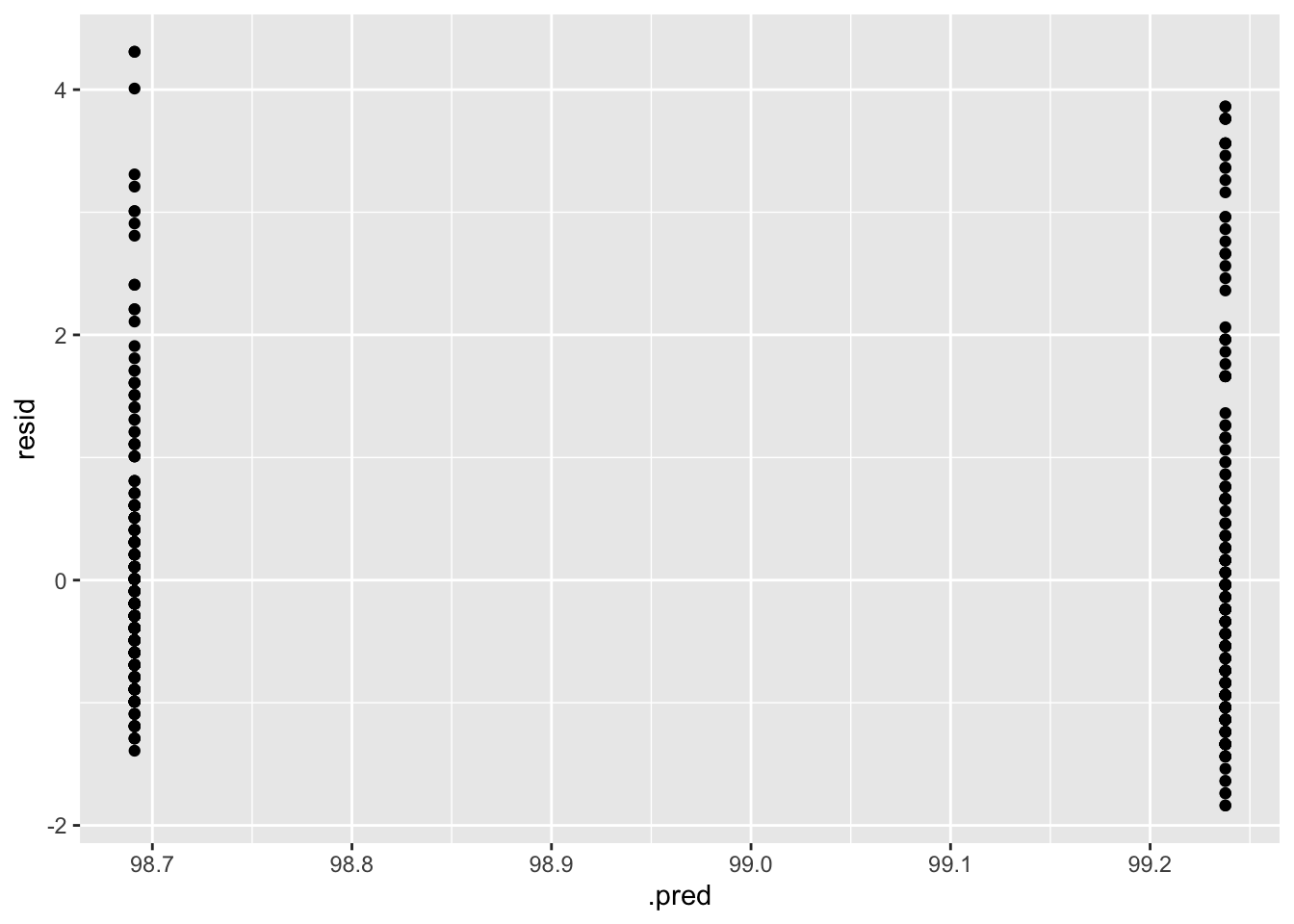

When looking at the autoplot of the results, it appears that a tree depth of one produces the lowest RMSE. We can see that this is the model that is chosen by looking at the extracted fit decision tree, which only goes down one level.

LASSO

The same basic steps for the tree model will be used for the LASSO model as well:

Define the model specification
Create a workflow
Create a tuning grid and tune the hyperparameters
Autoplot the results
Finalize the workflow
Fit the model to the training data
Estimate model performance with RMSE
Make diagnostic plots

# 1) define model spec 
lasso_tune_spec <- linear_reg(
  penalty = tune(), mixture = 1) %>% 
  set_engine('glmnet')
lasso_tune_spec

## Linear Regression Model Specification (regression)
## 
## Main Arguments:
##   penalty = tune()
##   mixture = 1
## 
## Computational engine: glmnet

# 2) workflow 
lasso_wflow <- workflow() %>% 
  add_model(lasso_tune_spec) %>% 
  add_recipe(temp_rec)


# 3) create tuning grid 
lasso_grid <- tibble(penalty = 10^seq(-4, -1, length.out = 30))

lasso_grid %>% top_n(-5)

## # A tibble: 5 × 1
##    penalty
##      <dbl>
## 1 0.0001  
## 2 0.000127
## 3 0.000161
## 4 0.000204
## 5 0.000259

lasso_grid %>% top_n(5)

## # A tibble: 5 × 1
##   penalty
##     <dbl>
## 1  0.0386
## 2  0.0489
## 3  0.0621
## 4  0.0788
## 5  0.1

# tune hyperparameters 
lasso_res <- lasso_wflow %>% 
  tune_grid(resample = cv5,
            grid = lasso_grid,
            control = control_grid(save_pred = T, verbose = T),
            metrics = metric_set(rmse))

# 4) autoplot the results 
lasso_res %>% autoplot()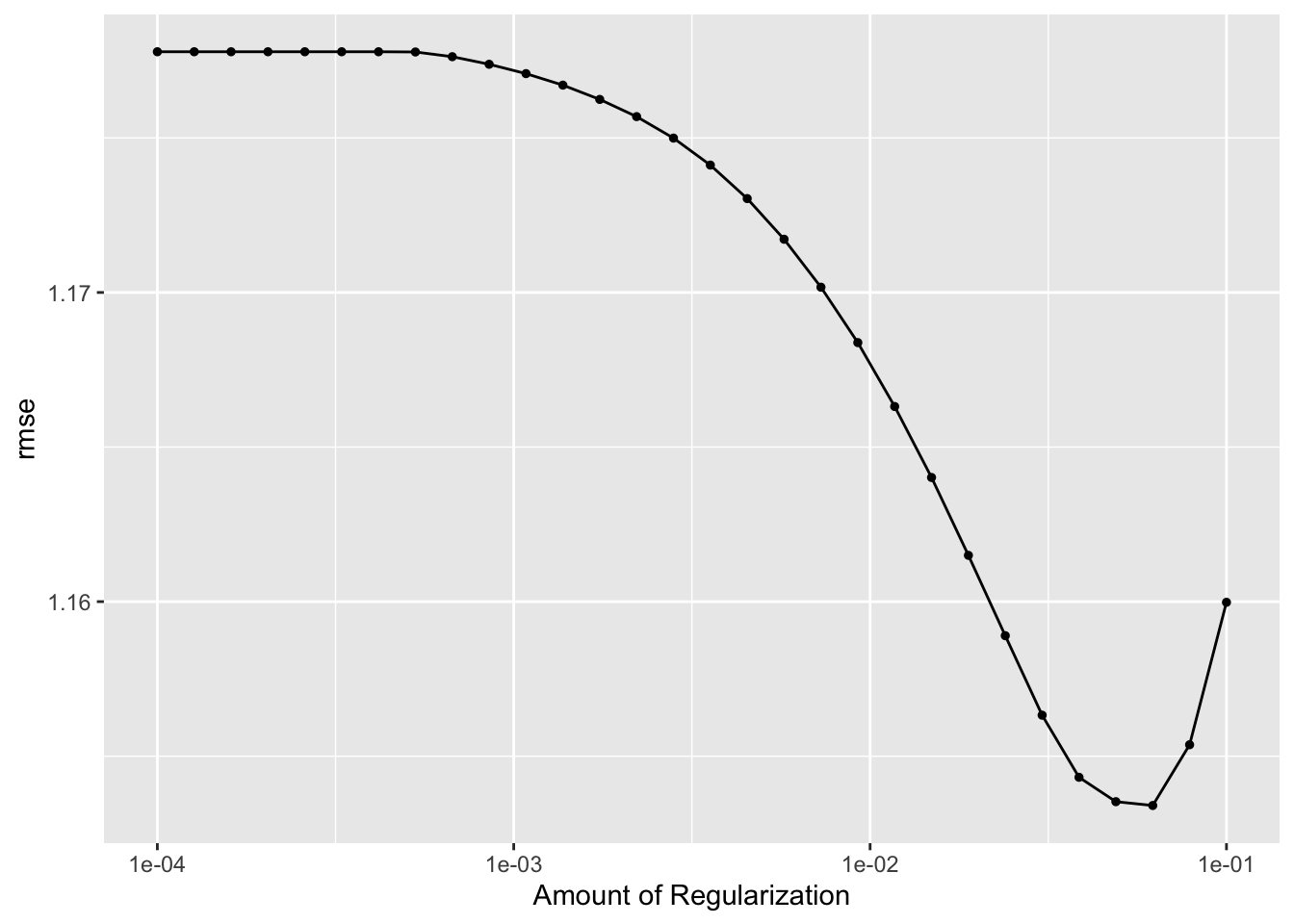

#5) finalize the workflow
# select best hyperparameter combination 
best_lasso <- lasso_res %>% 
  select_best()
best_lasso

## # A tibble: 1 × 2
##   penalty .config              
##     <dbl> <chr>                
## 1  0.0621 Preprocessor1_Model28

# finalize workflow 
best_lasso_wflow <- lasso_wflow %>% 
  finalize_workflow(best_lasso)

fit_best_lasso <- best_lasso_wflow %>% 
  fit(data = train_data)

#6) fit the model to the test data 
# Use a trained workflow to predict section using train data
predict(fit_best_lasso, new_data = train_data)

## # A tibble: 508 × 1
##    .pred
##    <dbl>
##  1  98.8
##  2  98.8
##  3  98.5
##  4  98.8
##  5  98.7
##  6  98.7
##  7  98.4
##  8  99.3
##  9  98.9
## 10  99.0
## # … with 498 more rows

# include predicted probabilities
aug_best_lasso <- augment(fit_best_lasso, new_data = train_data)

# estimate model performance with rmse 
lasso_rmse <- aug_best_lasso %>% 
  rmse(truth = BodyTemp, .pred) %>% 
  mutate(model = 'LASSO')
lasso_rmse

## # A tibble: 1 × 4
##   .metric .estimator .estimate model
##   <chr>   <chr>          <dbl> <chr>
## 1 rmse    standard        1.13 LASSO

# 8) Make diagnostic plots 
## view coefficient values vs penalty terms 
extract_fit_engine(fit_best_lasso) |> plot('lambda')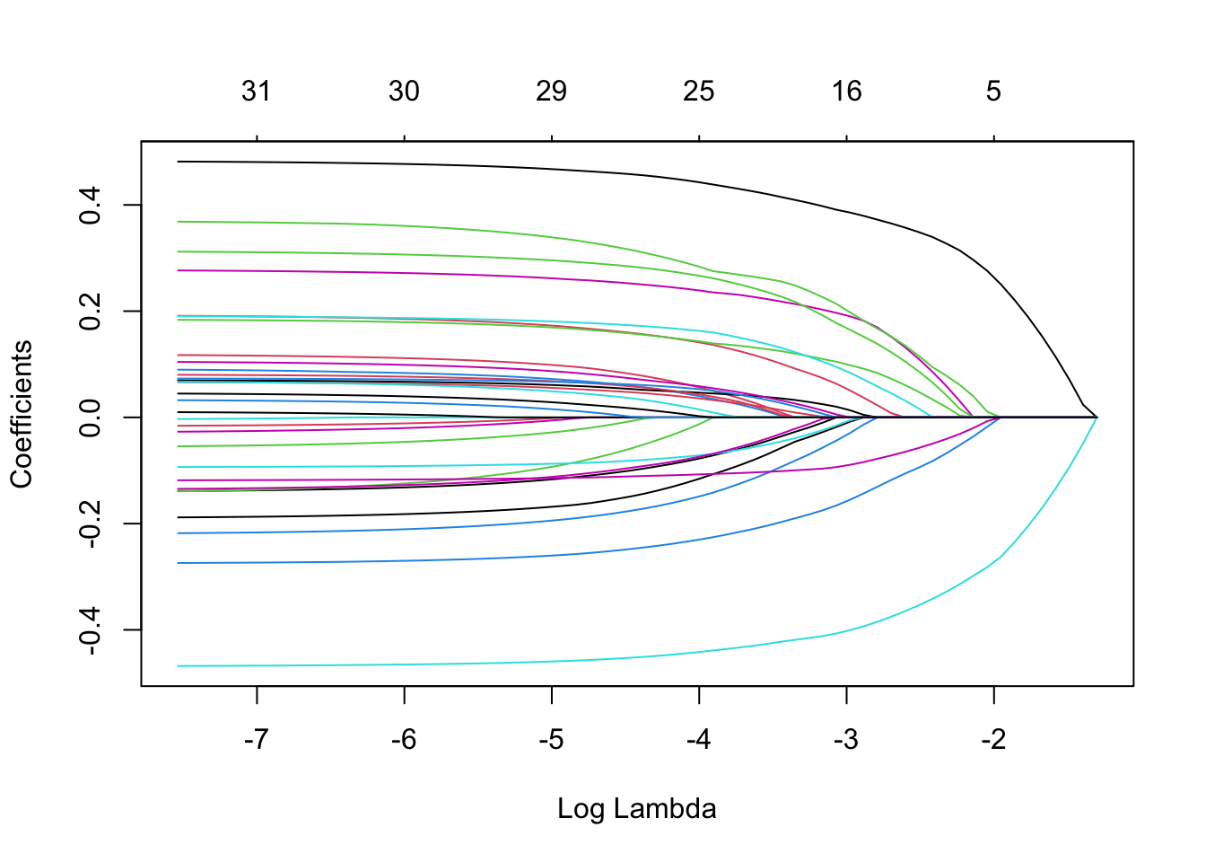

#plot actual vs fitted  
ggplot(data = aug_best_lasso, aes(x = .pred, y = BodyTemp)) +
  geom_point()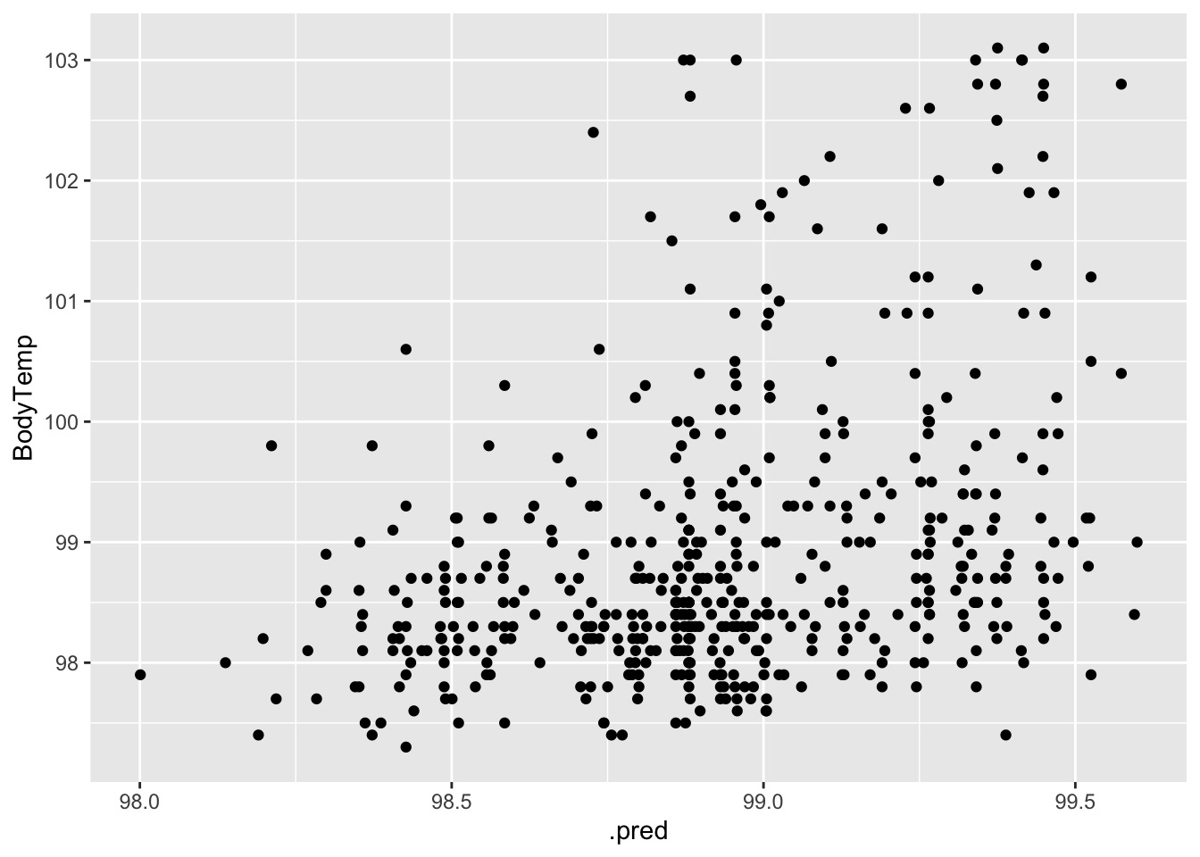

#plot residuals vs fitted 
aug_best_lasso %>% 
  mutate(resid = BodyTemp - .pred) %>% 
  ggplot(aes(x = .pred, y = resid)) +
  geom_point()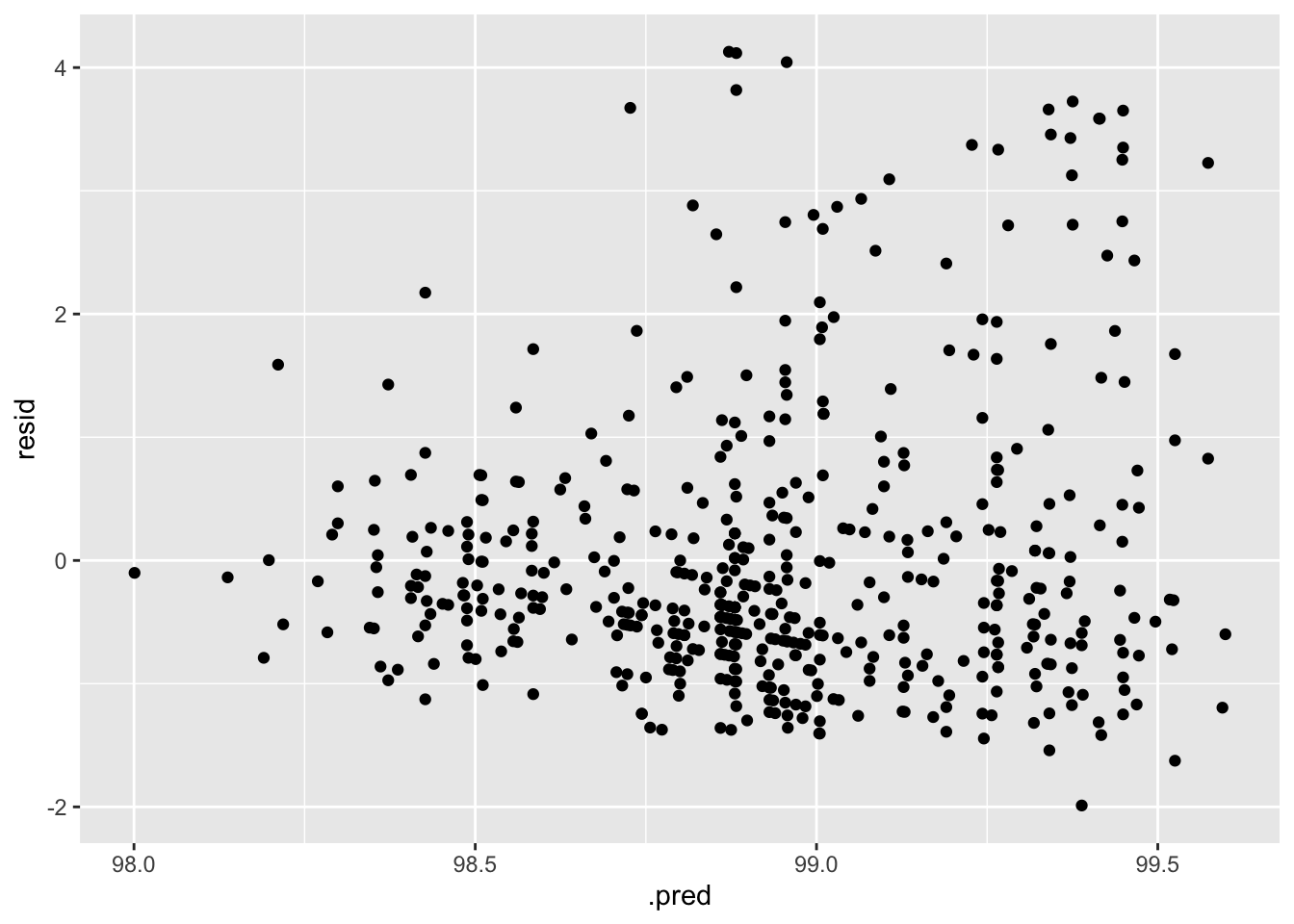

My biggest concern with this model is that the variance seems to increase with increasing temperature. Prediction accuracy also increases as temperature increases.

Random Forest

We’ll follow these same steps one last time!

Define the model specification
Create a workflow
Create a tuning grid and tune the hyperparameters
Autoplot the results
Finalize the workflow
Fit the model to the training data
Estimate model performance with RMSE
Make diagnostic plots

#cores <- parallel::detectCores()
#cores

# 1) define model spec 
forest_spec <-
  rand_forest(
    mtry = tune(),
    min_n = tune(),
    trees = 1000
    ) %>%
  set_engine('ranger', 
             num.threads = 1) %>%
  set_mode('regression')
forest_spec

## Random Forest Model Specification (regression)
## 
## Main Arguments:
##   mtry = tune()
##   trees = 1000
##   min_n = tune()
## 
## Engine-Specific Arguments:
##   num.threads = 1
## 
## Computational engine: ranger

# 2) workflow 
forest_wflow <- workflow() %>% 
  add_model(forest_spec) %>% 
  add_recipe(temp_rec)


# 3/4) create tuning grid/tune hyperparameters 
forest_spec %>% parameters()

## Collection of 2 parameters for tuning
## 
##  identifier  type    object
##        mtry  mtry nparam[?]
##       min_n min_n nparam[+]
## 
## Model parameters needing finalization:
##    # Randomly Selected Predictors ('mtry')
## 
## See `?dials::finalize` or `?dials::update.parameters` for more information.

forest_res <- forest_wflow %>% 
  tune_grid(resample = cv5,
            grid = 25,
            metrics = metric_set(rmse),
            control = control_grid(save_pred = T, verbose = T))


forest_res %>% show_best(metric = "rmse")

## # A tibble: 5 × 8
##    mtry min_n .metric .estimator  mean     n std_err .config              
##   <int> <int> <chr>   <chr>      <dbl> <int>   <dbl> <chr>                
## 1     6    35 rmse    standard    1.16    25  0.0166 Preprocessor1_Model20
## 2     8    38 rmse    standard    1.17    25  0.0167 Preprocessor1_Model16
## 3     2    16 rmse    standard    1.17    25  0.0167 Preprocessor1_Model01
## 4     3    10 rmse    standard    1.17    25  0.0163 Preprocessor1_Model14
## 5    10    28 rmse    standard    1.17    25  0.0167 Preprocessor1_Model23

# 5) autoplot the results 
forest_res %>% autoplot()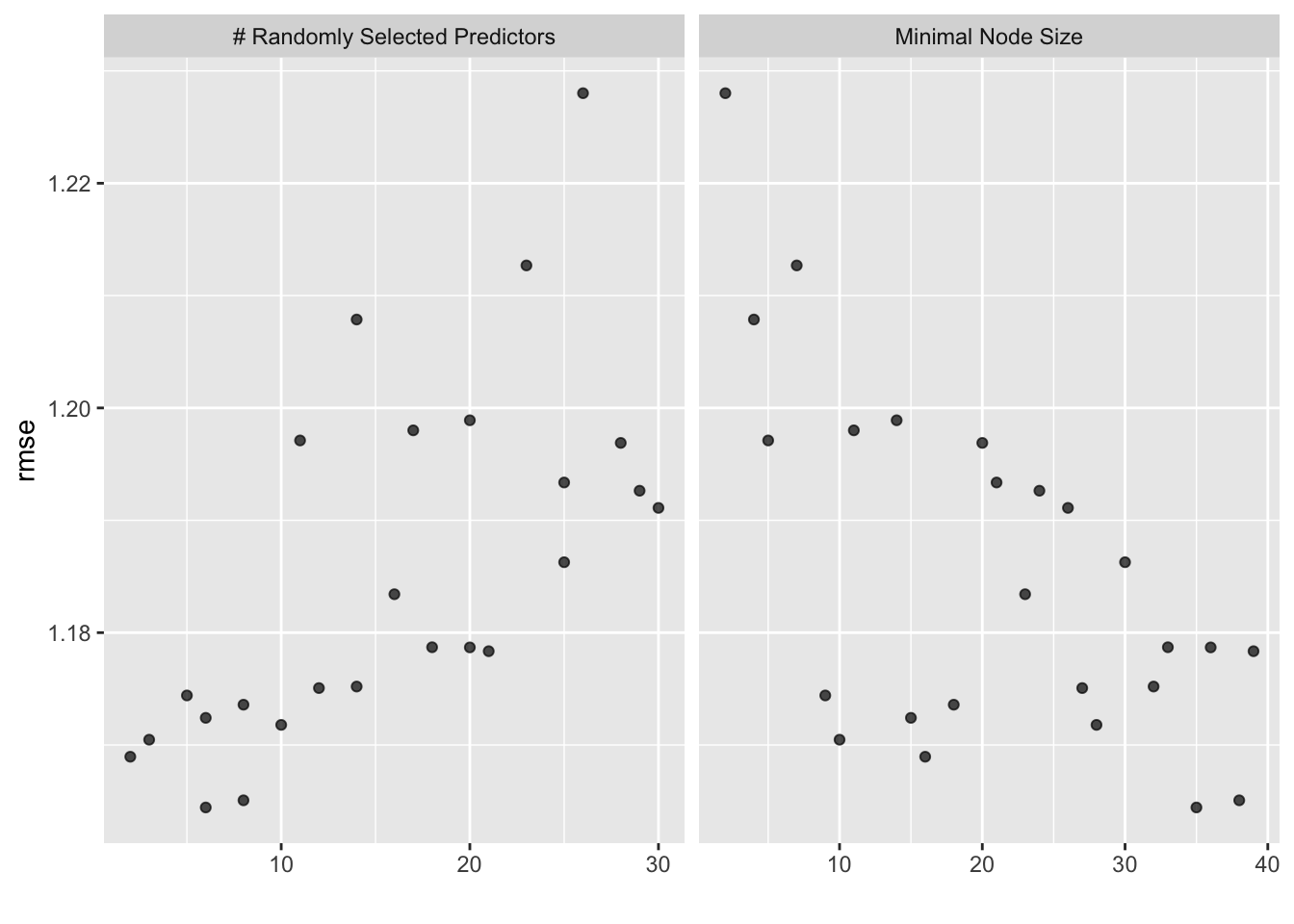

# select best hyperparameter combination 
best_forest <- forest_res %>% 
  select_best() 
best_forest

## # A tibble: 1 × 3
##    mtry min_n .config              
##   <int> <int> <chr>                
## 1     6    35 Preprocessor1_Model20

# finalize workflow 
best_forest_wflow <- forest_wflow %>% 
  finalize_workflow(best_forest)

fit_best_forest <- best_forest_wflow %>% 
  fit(data = train_data)

# Use a trained workflow to predict section using train data
predict(fit_best_forest, new_data = train_data)

## # A tibble: 508 × 1
##    .pred
##    <dbl>
##  1  98.7
##  2  98.6
##  3  98.7
##  4  98.7
##  5  98.8
##  6  98.6
##  7  98.3
##  8  99.1
##  9  98.8
## 10  98.9
## # … with 498 more rows

# include predicted probabilities
aug_best_forest <- augment(fit_best_forest, new_data = train_data)

# estimate model performance with rmse 
forest_rmse <- aug_best_forest %>% 
  rmse(truth = BodyTemp, .pred) %>% 
  mutate(model = 'Random Forest')
forest_rmse

## # A tibble: 1 × 4
##   .metric .estimator .estimate model        
##   <chr>   <chr>          <dbl> <chr>        
## 1 rmse    standard        1.03 Random Forest

# 8) Make diagnostic plots 

#plot actual vs fitted  
ggplot(data = aug_best_forest, aes(x = .pred, y = BodyTemp)) +
  geom_point()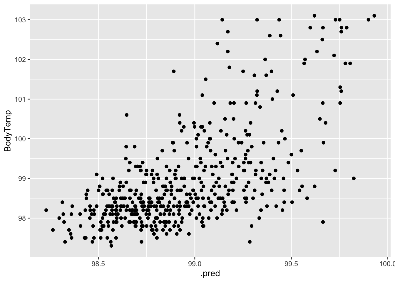

#plot residuals vs fitted 
aug_best_forest %>% 
  mutate(resid = BodyTemp - .pred) %>% 
  ggplot(aes(x = .pred, y = resid)) +
  geom_point()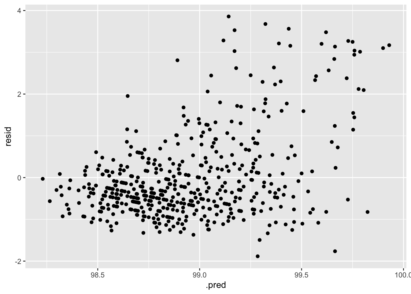

These diagnostic plots looks a little better than those of the LASSO model. The RMSE is lower as well. These things indicate this is a better model for this analysis.

Model Selection

In order to choose the best performing model, I will look at all of the RMSEs together. The model with the lowest RMSE will be the one I fit to the test data.

#view RMSEs of all four models 
knitr::kable(rbind(null_rmse, tree_rmse, lasso_rmse, forest_rmse))

.metric	.estimator	.estimate	model
rmse	standard	1.163334	Null Model
rmse	standard	1.178367	Regression Tree
rmse	standard	1.131147	LASSO
rmse	standard	1.026835	Random Forest

The random forest model performed far better than the other three, as evidenced by the lowest RMSE, so I will fit the test data to this model.

Final Model Fit to Test Data

forest_final <- best_forest_wflow %>% 
  last_fit(data_split) 


# Use a trained workflow to predict section using test data
forest_final %>% 
  collect_predictions()

## # A tibble: 222 × 5
##    id               .pred  .row BodyTemp .config             
##    <chr>            <dbl> <int>    <dbl> <chr>               
##  1 train/test split  99.1     2    100.  Preprocessor1_Model1
##  2 train/test split  99.0     4     98.8 Preprocessor1_Model1
##  3 train/test split  99.7    11     98.2 Preprocessor1_Model1
##  4 train/test split  99.4    12     97.9 Preprocessor1_Model1
##  5 train/test split  98.7    14    102.  Preprocessor1_Model1
##  6 train/test split  99.4    17     99.3 Preprocessor1_Model1
##  7 train/test split  99.4    25     97.8 Preprocessor1_Model1
##  8 train/test split  99.4    27     99.5 Preprocessor1_Model1
##  9 train/test split  99.2    29     99.7 Preprocessor1_Model1
## 10 train/test split  99.2    32     98.8 Preprocessor1_Model1
## # … with 212 more rows

# include predicted probabilities
aug_final_forest <- augment(forest_final)

# estimate model performance with rmse 
aug_final_forest %>% 
  rmse(truth = BodyTemp, .pred)

## # A tibble: 1 × 3
##   .metric .estimator .estimate
##   <chr>   <chr>          <dbl>
## 1 rmse    standard        1.18

# 8) Make diagnostic plots 
#plot actual vs fitted  
ggplot(data = aug_final_forest, aes(x = .pred, y = BodyTemp)) +
  geom_point()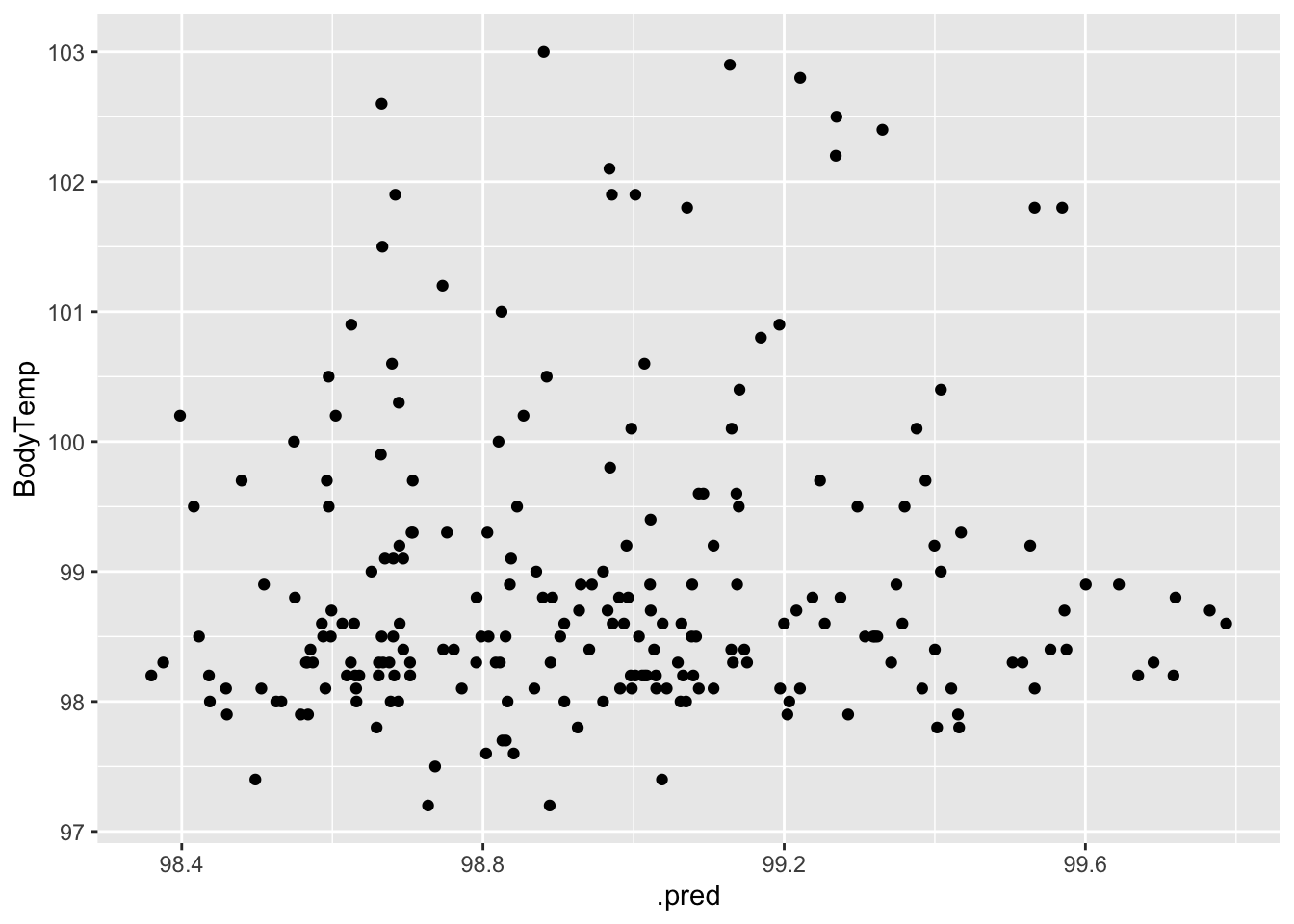

#plot residuals vs fitted 
aug_final_forest %>% 
  mutate(resid = BodyTemp - .pred) %>% 
  ggplot(aes(x = .pred, y = resid)) +
  geom_point()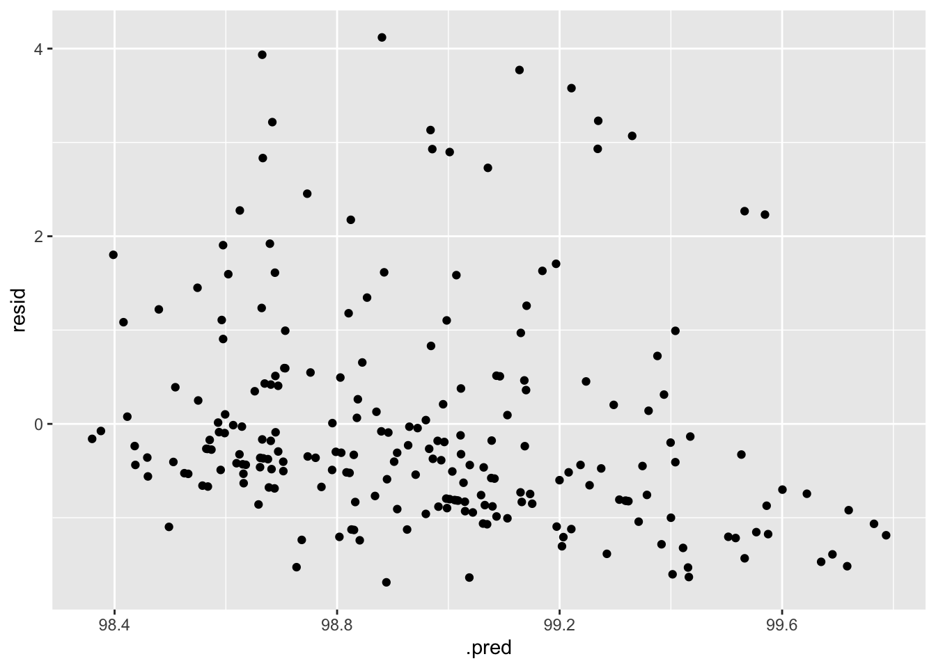

When fit to the test data, the model did not perform quite as well as it did when fit to the train data, but this is not too surprising. The diagnostic plots also indicate increased variance.

Analysis and Model Fitting Exercise